Twitter Sentiment Through the Lens of Kanye West
by Patrick Larsen
Note: arrow symbols are difficult to transport from RStudio into Brackets, so certain assignment operators (particularly ones that point left) have been replaced with a simple =.
I am a news guy. If you've read my previous reports for this class, you likely already know this. In some ways, I'm lucky - in the past two years or so, there has been more than enough fascinating news to go around. However, precisely because of this, the news has occasionally become grating, even to me. And then Kanye West reactivated his Twitter account. Suddenly, we saw a master provocateur ending a long-standing public silence with controversial tweet after controversial tweet. In many ways, the story was so dense that it was hard to make sense of - but that didn't stop a massive public reaction.
Hypothesis:
If we compare the sentiment of tweets about Kanye West and Twitter as a whole, then we will find that the sentiment of tweets about West are notably lower.*
*When writing my hypothesis, I decided it would be best to include the whole of Twitter as a control. It's not hard to gather the data from the Twitter API, and I can easily run a few different days to find a better average.
I tested this using data gathered from the Twitter API. It took some doing, and ultimately I was not able to retrieve the best data for a time-based analysis with the level of access that I had. That said, it is possible to gain more complete access to the API through services like Sysomos. Free trials are available on their website, but they are limited to one trial per company, which is why I was not able to access one for myself.
We'll start with the packages for retrieving data from the Twitter API. Note that because the rtweet package is not on CRAN, we have to call it with a devtools request.
library(devtools)
devtools::install_github("mkearney/rtweet")
library(rtweet)
library(tidyverse)
library(tidytext)
Now that we have our packages loaded, we can use it to access what we're looking for in the API. In this case - tweets including "kanye." This was difficult, because I wanted to find a way to limit the API's responses by date, and I found no successful way to do so with actual dates. What I settled on was using the max_id command in rtweet. This allows you to specify a single tweet as a cap, so that none of the tweets you retrieve will come after it. This is the code, starting with a call for West's twitter stream to use as reference:
kanyeTwitter = get_timeline(
"kanyewest", n=18000, retryonratelimit = TRUE, lang = "en")
kanye0430 = search_tweets(
q = "kanye", n = 18000, max_id = 991092016195911680, retryonratelimit = FALSE)
This gave me the data for March 30th. I repeated this process using the appropriate tweet ID from March 25th to April 5th. Unfortunately, due to the API limitations I mentioned earlier, I was not able to go farther back than that. Sysomos would help with this.
Next, I wanted to analyze sentiment for each of the dates, but I was not necessarily interested in the number of positive words vs. negative words, at least at this point. So, I settled on the AFINN lexicon, which assigns each word with a score from -5 to 5, negative numbers being of negative sentiment, positive numbers being of positive sentiment. But before we do any of this, we need to clean the data into a two-variable dataframe:
cleaned_0430 = kanye0430 %>%
mutate(text = gsub("http://*|https://*)", "", text))
data("stop_words")
cleaned_0430_2 = cleaned_0430 %>%
dplyr::select(text) %>%
unnest_tokens(word, text) %>%
anti_join(stop_words)
That's all you need to clean your data for this process. Unnest_tokens will separate the tweets into individual words, and stop_words will remove common but inconsequential words like "the," or "and." Next, let's analyze with AFINN. We'll need to install/load the scales package from CRAN to access AFINN.
library(scales)
afinn0430 = cleaned_0430_2 %>%
inner_join(get_sentiments("afinn")) %>%
summarise(sentiment = sum(score)) %>%
mutate(method = "AFINN")
afinn0430mean = cleaned_0430_2 %>%
inner_join(get_sentiments("afinn")) %>%
summarise(sentiment = mean(score)) %>%
mutate(method = "AFINN")
I started by running the first line for each date to find the sum of sentiment, but that ended up making an innacurate visualisation of the data. The number of tweets I retrieved from each date varied, sometimes by thousands of data points, meaning that once the data was split into individual words, there was just no way to accurately compare sums. So, I reran everything with the second line. This gave me the mean sentiment for a tweet from each day, which is much more uniform. I organized my data in a CSV and ran it with ggplot2:
library(ggplot2)
ggplot(kanyeResponseSentiment_afinn4, aes(Date, AFINNscore)) +
geom_point() +
ggtitle("Average Sentiment of Tweets about Kanye West Over Time") +
theme(plot.title = element_text(size = 12, face = "bold",
margin = margin(10, 0, 10, 0))) +
theme(axis.text.x=element_text(angle=60, size=10, vjust=0.5)) +
ylim(c(-1.5, 0))
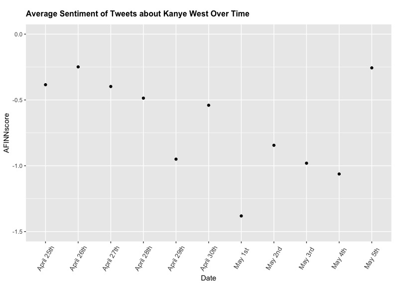
That's not bad! We have a pretty clear graph - a line graph would be better, but ggplot2 refused. I'm not totally sure why. Anyway, this does the job well enough. Now, let's get started on our control. The process for this will be basically identical, except we don't really need to recreate the above plot. Instead, let's just find the mean for one API call (~18,000 tweets).
cleaned_twitter = twitter %>%
mutate(text = gsub("http://*|https://*)", "", text))
cleaned_twitter_2 = cleaned_twitter %>%
dplyr::select(text) %>%
unnest_tokens(word, text) %>%
anti_join(stop_words)
afinntwittermean = cleaned_twitter_2 %>%
inner_join(get_sentiments("afinn")) %>%
summarise(sentiment = mean(score)) %>%
mutate(method = "AFINN")
When we run that, we see that the mean is 0.178 - putting it squarely above all Kanye-related averages, which never made it over 0. It's worth noting that the sentiment of West's Twitter account up until May 5th is a whopping 0.849, putting him even higher above the average.
So, that's my hypothesis proven. Tweets including the word "Kanye" tend to be more negative than tweets on average. But why stop there? Let's dig into the data a little bit more.
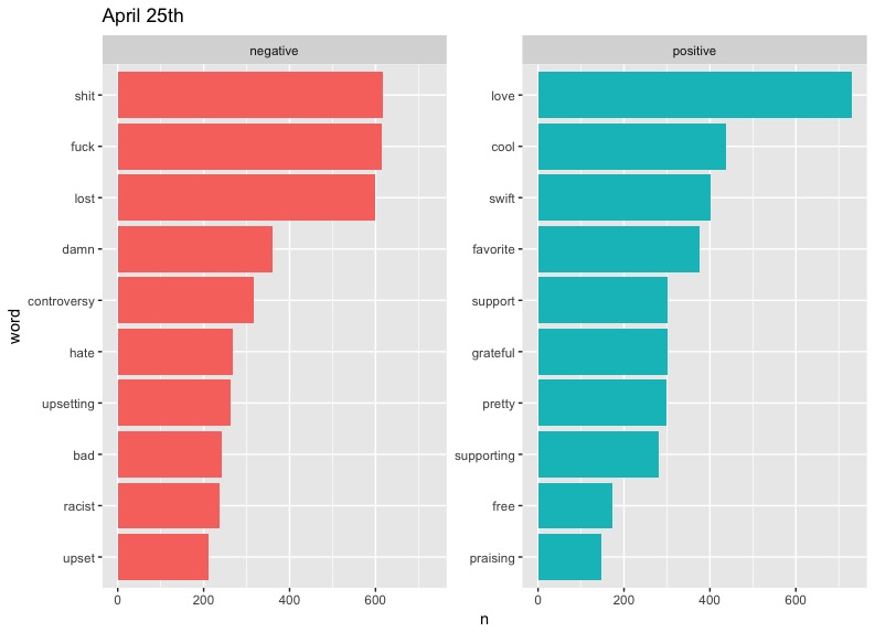
First, let's continue organizing the data to run Bing sentiment tests with them. Maybe we'll find an interesting trend.
cleaned_0430_2 %>%
filter(!word %in% c("rt", "t.co", "https", "trump")) -> cleaned_0430_3
cleaned_0430_3 %>%
count(word, sort = TRUE) %>%
mutate(word = reorder(word, n)) -> cleaned_0430_4
kanye0430_word_counts = cleaned_0430_3 %>%
inner_join(get_sentiments("bing")) %>%
count(word, sentiment, sort = TRUE) %>%
ungroup()
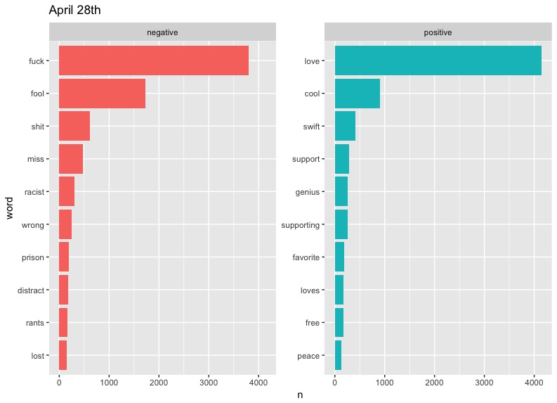
kanye0430_word_counts %>%
group_by(sentiment) %>%
top_n(10) %>%
ungroup() %>%
mutate(word = reorder(word, n)) %>%
ggplot(aes(word, n, fill = sentiment)) +
ggtitle("March 30th") +
geom_col(show.legend = FALSE) +
facet_wrap(~sentiment, scales = "free_y") +
coord_flip()
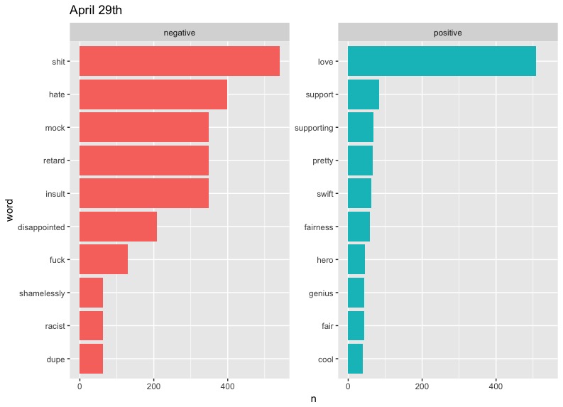
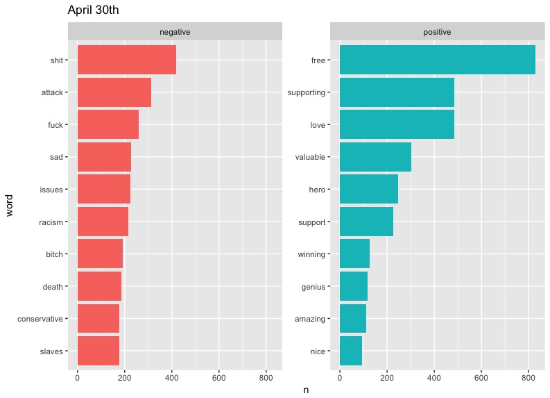
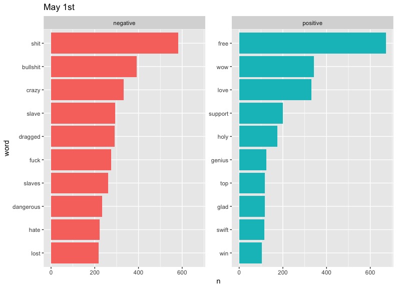
Now run for each date, and plot.
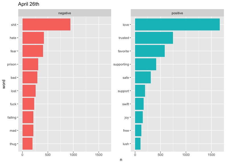
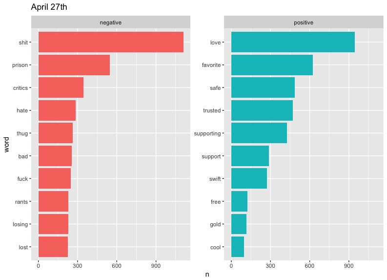
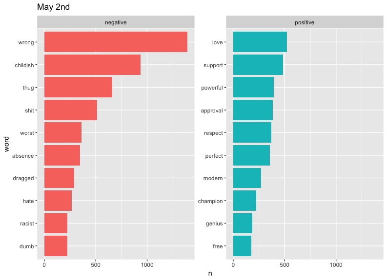
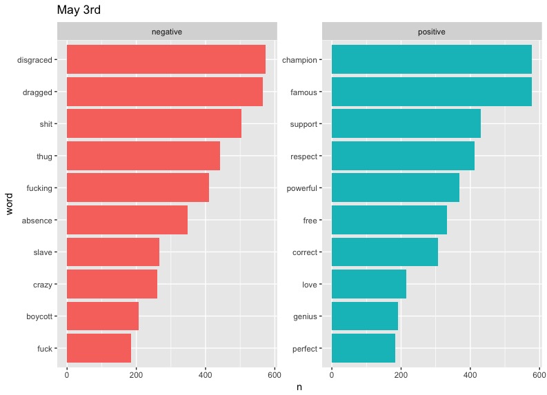
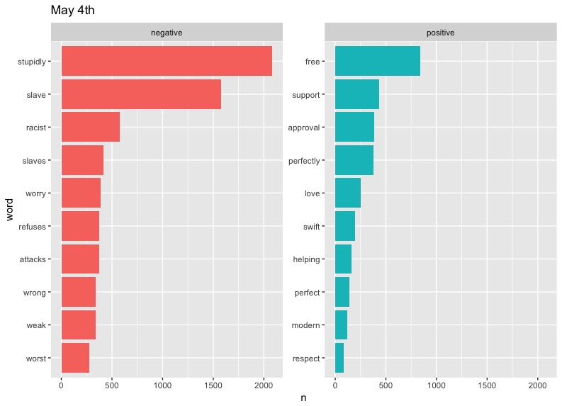
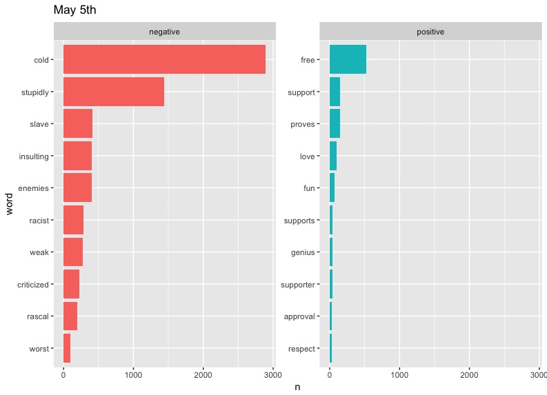
There are some clear problems with our data here, such as "cold" taking such a massive slice on April 5th - something tells me that there is a small likelihood that "cold" would be the diss of choice on Twitter. As it turns out, West has a song called "Cold," but even then, we can't be sure of the reason this word appears so much. Also notable are the high occurrences of "Champion" and "Famous" on May 3rd. These can be explained by the fact that they are names of two of West's most popular songs. We could limit the data to exclude these words if we wanted to, but these graphs will do.
In terms of trends, perhaps the most notable one is that of "love." West included the word regularly in his tweets, preaching about the power of love in a fearful world. It's interesting to see this generally drop out of the top half of positive words represented on later dates. This may say something about people's response to Kanye's message becoming more negative or perhaps less focused over time.
Let's look at the same chart with data from Kanye's Twitter feed until May 5th.
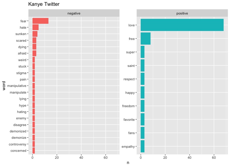
Wouldn't you know it, the number one positive word on West's Twitter is "love." This goes right in line with the prevalence of the word in tweets about West.
While we're here, lets try out another visualisation. Let's run the following, using the data from West's feed:
install_github("lchiffon/wordcloud2")
library(wordcloud2)
wordcloud2(cleaned_Feed_4, size = 2, shape = "oval")
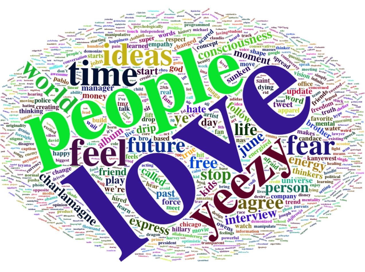
Well, doesn't that look nice. It would probably be wise to limit the data to the top 100 words, but at least for this one and its limited data, it's nice to see it so filled out. Next, let's cherry pick a date, we'll say April 29th, and we can make another wordcloud from responses for comparison. To do this, we'll have to do some additional work with the dataset:
cleaned_0430_5 = cleaned_0430_3 %>%
inner_join(get_sentiments("bing")) %>%
ungroup()
cleaned_0430_6 = cleaned_0430_5 %>%
dplyr::select(word)
cleaned_0430_6 %>%
count(word, sort = TRUE) %>%
mutate(word = reorder(word, n)) -> cleaned_0430_7
I'll be honest, there's probably a much easier way to do this, but it worked with the iterations I already had. Anyway, just run the same wordcloud code as before, and here's the final product:
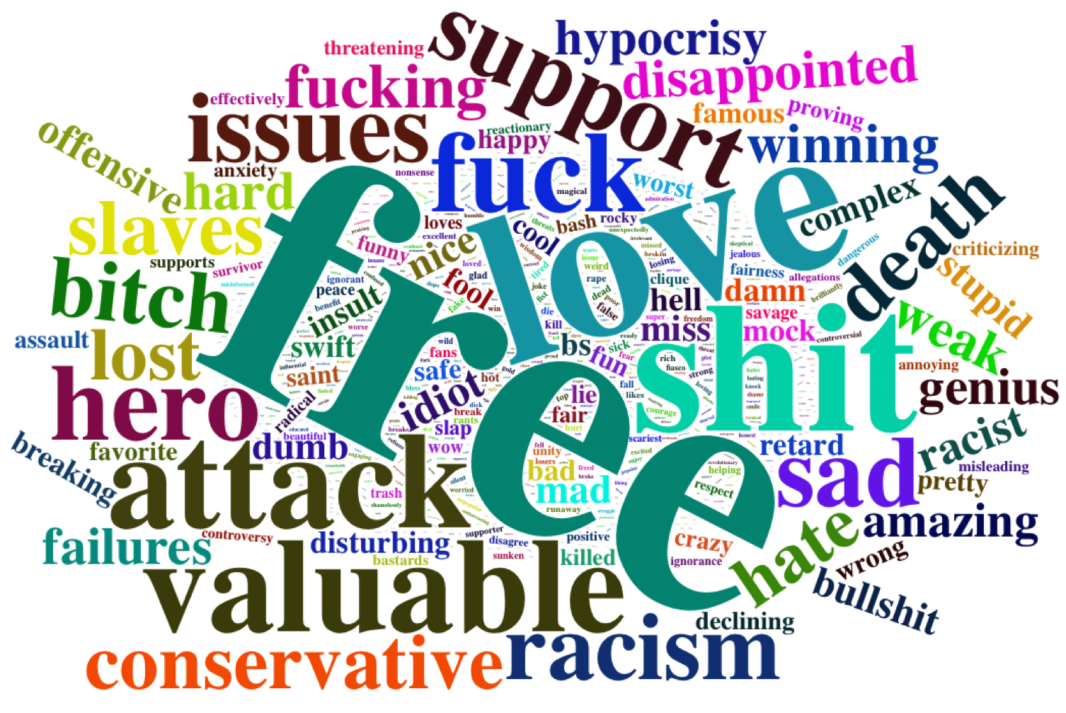
That looks considerably less nice. A mixed bag, at best.
In closing, my hypothesis was proved, and we had the means to make some fun visualisations that tell us exactly why that is. Twitter is a nice place to gather data from, because of its indefinite nature. With diligent work, you could track sentiment in response to West's tweets for each day from now until he stops tweeting, and you could do the same with any other public figure. Perhaps this negative sentiment will be a predictor for the outcome of Kanye's inevitable presidential run - or maybe it will be completely off. We'll have to wait and see.