Does Toro Y Moi's Music Get Happier?
Joseph Henry-Penrose for COM 329
Introduction:
Toro Y Moi is the longtime project of Chaz Bear (formerly Chaz Bundick). Toro Y Moi is often associated with chillwave, house, and psychedelic rock. Needless to say, Chaz and his band have an extremely varied discography. Chaz embraces change in a way that many other artists are unable to fathom. He has jumped from genre to genre and topic to topic. After his slightly disappointing release Boo Boo in 2017, I wondered if Bear had a great deal of artistic exploration left in Toro Y Moi. Thankfully, he has bounced back with his new release Outer Peace. The new record made me think about the nostalgia-drenched albums that Chaz has been releasing for a few years and forced me to question if his music has become happier. So, what better way to find out than a statistical analysis.
My Hypothesis: Sentiment analysis, valence, and the lyrics themselves will show that Toro Y Moi's music gets happier with each new release.
Lyric data was collected from the Genius API through GeniusR and data on albums was collected using Spotify's API with SpotifyR. A plethora of packages have been used for analysis and data cleaning.
There are nine Toro Y Moi albums, but one is a live album and two other have little-to-no lyrical data on Genius, leading to errors. Due to this, we'll stick with the six most recent albums; Underneath The Pine, June 2009, Anything In Return, What For?, Boo Boo, and Outer Peace.
If you're not familiar with Toro Y Moi's Music, have a listen below:
Set Up:
library(tidyverse)
library(tidytext)
install.packages("devtools")
library(devtools)
devtools::install_github('charlie86/spotifyr')
install.packages('spotifyr')
library(spotifyr)
Sys.setenv(SPOTIFY_CLIENT_ID = ‘YOUR KEY’)
Sys.setenv(SPOTIFY_CLIENT_SECRET = ‘YOUR KEY’)
access_token <- get_spotify_access_token()
devtools::install_github("josiahparry/genius")
library(genius)
library(knitr)
install.packages("ggplot2")
library(ggplot2)
install.packages("ggjoy")
library(ggjoy)
install.packages("ggridges")
library(ggridges)
library(dplyr)
install.packages("tm")
library(tm)
library(RColorBrewer)
install.packages('wordcloud2')
library(wordcloud2)
install.packages("data.table")
library(data.table)
Joy Plot:
Before we can look into patterns, let's have an overall look at joy through each album. With Spotify's API, you can see the valence–a measure of happiness–of each song. This can then be graphed in order of songs to show the general arch and amounts of happiness throughout.
I used the spotify API and ggjoy, an older version of ggridges, to plot map of valence.
TYM_joy <- get_artist_audio_features('toro y moi’)
TYM_joy <- filter(TYM_joy, album_name %in% c("What For?", "Underneath The Pine", "Outer Peace", "June 2009", "Boo Boo", "Anything In Return”))
TYM_joy %>%
arrange(-album_release_year) %>%
select(track_name, valence) %>%
head(5) %>%
kable()
ggplot(TYM_joy, aes(x = valence, y = album_name)) +
geom_joy() +
theme_joy() +
ggtitle("Joyplot of Toro Y Moi's joy distributions",
subtitle = "Based on valence pulled from Spotify's Web API with spotifyr")
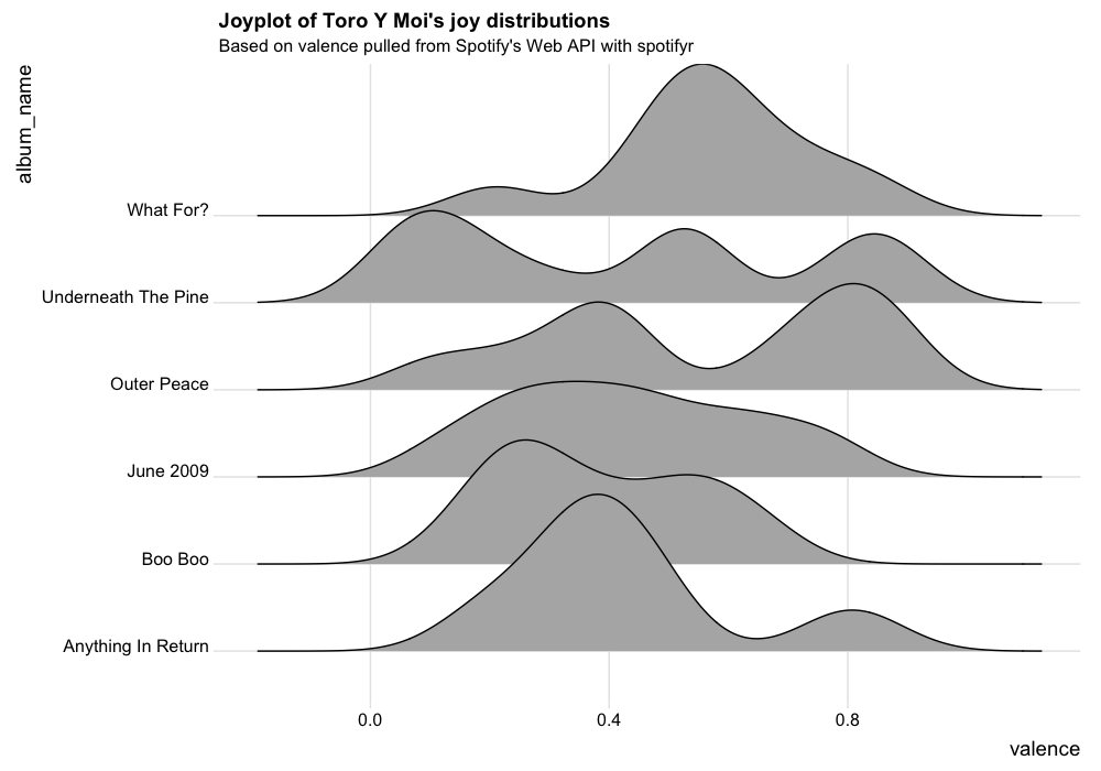
Ridge plot of valence by song, grouped by album
Looking at this, we can see that none of Toro Y Moi's albums have a unifying feel to them with some having one single joyful build and others cresting two or even three times. This gives us a basic understanding of how joyful each album is, with early albums Underneath the Pine and June 2009 showing lower levels of joy when compared to the later albums What For? and Outer Peace.
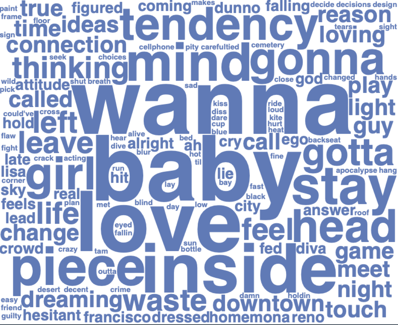
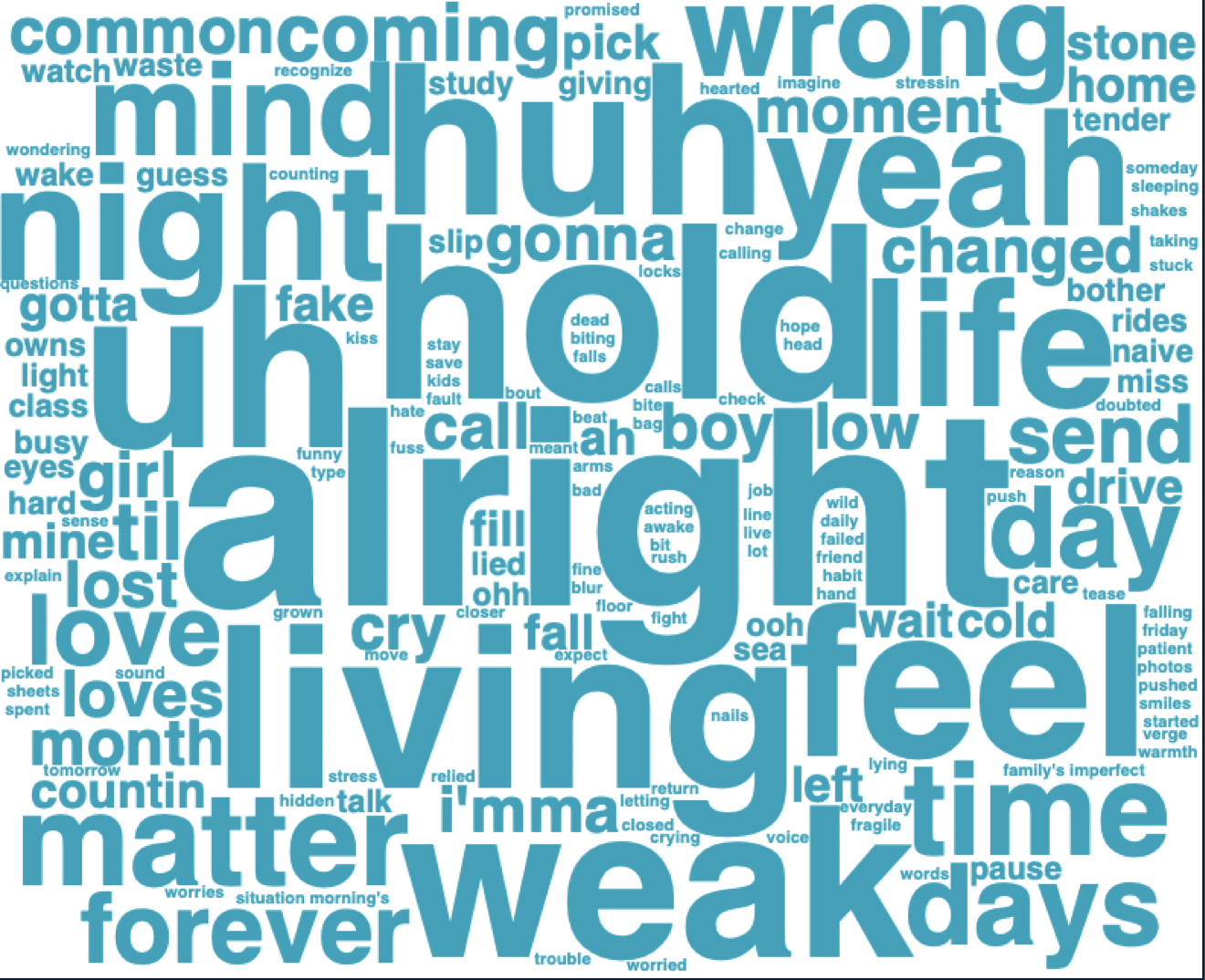
Word Clouds and Most Used Words
After gaining the basic understanding of the joy in each album, I wanted to see what the most common words in each album were to see if there were any standout differences. First, we need to import the lyrics for each album.
TYM_Left_Alone_At_Night <- genius_album(artist = "Toro Y Moi", album = "Left-alone-at-night")
TYM_Outer_Peace <- genius_album(artist = "Toro Y Moi", album = "Outer Peace")
TYM_Boo_Boo <- genius_album(artist = "Toro Y Moi", album = "Boo Boo")
TYM_What_For <- genius_album(artist = "Toro Y Moi", album = "What For?")
TYM_Anything_In_Return <- genius_album(artist = "Toro Y Moi", album = "Anything In Return")
TYM_June_2009 <- genius_album(artist = "Toro Y Moi", album = "June 2009")
TYM_Underneath_The_Pine <- genius_album(artist = "Toro Y Moi", album = "Underneath The Pine")
TYM_Causers_Of_This <- genius_album(artist = "Toro Y Moi", album = "Causers of This")
#Adding album names to each table
TYM_Outer_Peace['Album_Name'] <- "Outer Peace"
TYM_Boo_Boo['Album_Name'] <- "Boo Boo"
TYM_What_For['Album_Name'] <- "What For?"
TYM_Anything_In_Return['Album_Name'] <- "Anything In Return"
TYM_June_2009['Album_Name'] <- "June 2009"
TYM_Underneath_The_Pine['Album_Name'] <- "Underneath The Pine"
#Outer Peace
TYM_Outer_Peace_Lyrics_Count <- TYM_Outer_Peace %>% unnest_tokens(word, lyric) %>%
anti_join(stop_words, by = 'word') %>%
count(word) %>%
arrange(-n) %>%
na.omit(TYM_Outer_Peace_Lyrics_Count)
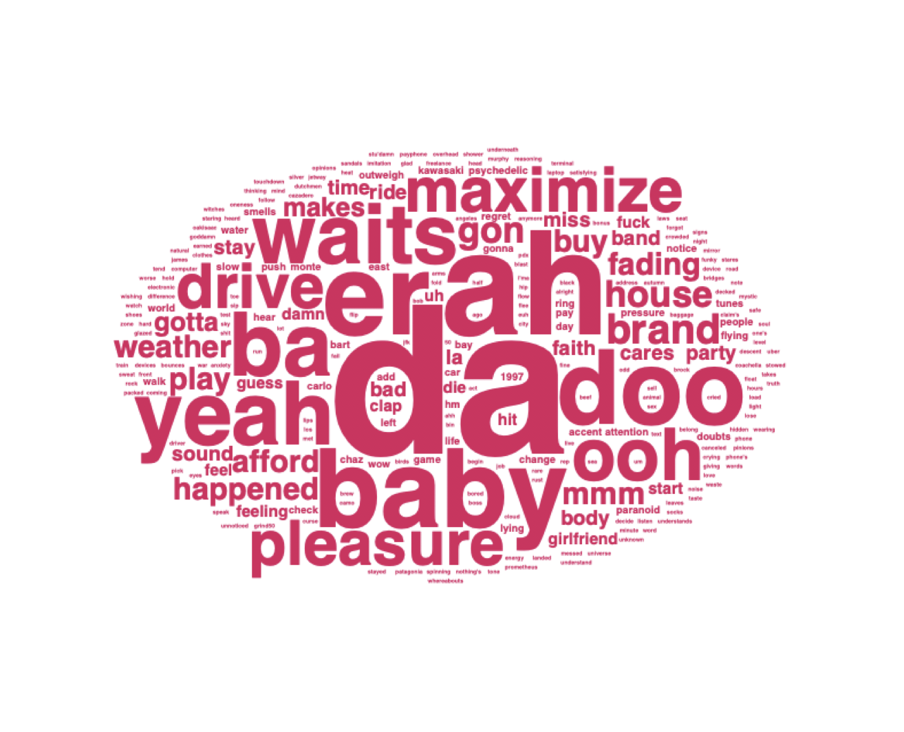
wordcloud2(TYM_Outer_Peace_Lyrics_Count, fontFamily = 'Helvetica', color = '#D81E5E',
minRotation = 0, maxRotation = 0, shape = 'rectangle')
ggplot(TYM_Outer_Peace_Lyrics_Count %>% head(15), aes(x=reorder(word, -n), y=n)) +
geom_bar(stat="identity", position="identity", fill ='#D81E5E') +
geom_hline(yintercept = 0, size = 1, colour="#333333") +
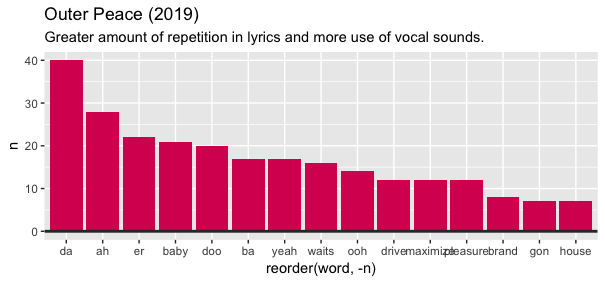
labs(title="Outer Peace (2019)",
subtitle = "Greater amount of repetition in lyrics and more use of vocal sounds.")
#Boo Boo
TYM_Boo_Boo_Lyrics_Count <- TYM_Boo_Boo %>% unnest_tokens(word, lyric) %>%
anti_join(stop_words, by = 'word') %>%
count(word) %>%
arrange(-n) %>%
na.omit(TYM_Boo_Boo_Lyrics_Count)
wordcloud2(TYM_Boo_Boo_Lyrics_Count, fontFamily = 'Helvetica', color = '#5C79BB', minRotation = 0, maxRotation = 0, shape = 'rectangle')
ggplot(TYM_Boo_Boo_Lyrics_Count %>% head(15), aes(x=reorder(word, -n), y=n)) +
geom_bar(stat="identity", position="identity", fill ='#5C79BB') +
geom_hline(yintercept = 0, size = 1, colour="#333333") +
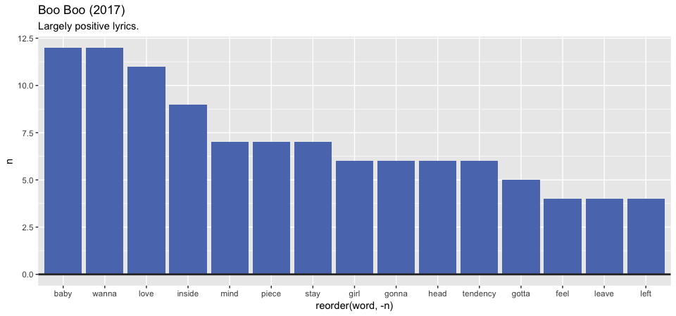
labs(title="Boo Boo (2017)",
subtitle = "Largely positive lyrics.")
#What For?
TYM_What_For_Lyrics_Count <- TYM_What_For %>% unnest_tokens(word, lyric) %>%
anti_join(stop_words, by = 'word') %>%
count(word) %>%
arrange(-n) %>%
na.omit(TYM_What_For_Lyrics_Count)
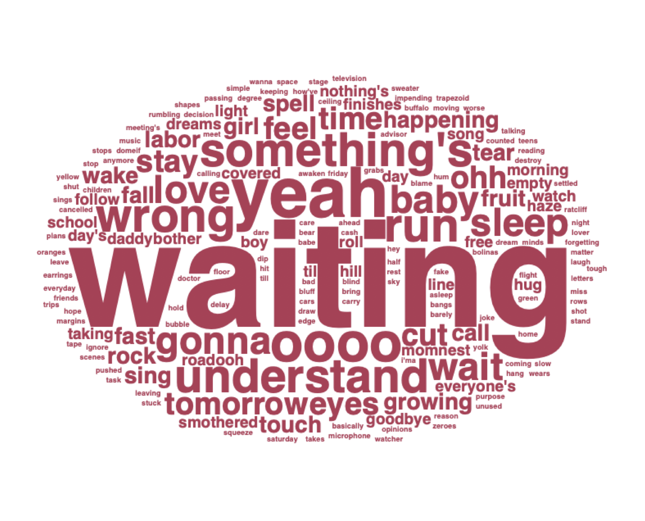
wordcloud2(TYM_What_For_Lyrics_Count, fontFamily = 'Helvetica', color = '#B13955', minRotation = 0, maxRotation = 0, shape = 'rectangle')
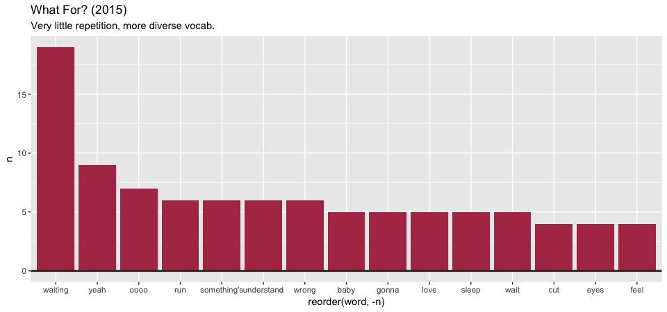
ggplot(TYM_What_For_Lyrics_Count %>% head(15), aes(x=reorder(word, -n), y=n)) +
geom_bar(stat="identity", position="identity", fill ='#B13955') +
geom_hline(yintercept = 0, size = 1, colour="#333333") +
labs(title="What For? (2015)",
subtitle = "Very little repetition, more diverse vocab.")
#Anything In Return
TYM_Anything_In_Return_Lyrics_Count <- TYM_Anything_In_Return %>% unnest_tokens(word, lyric) %>%
anti_join(stop_words, by = 'word') %>%
count(word) %>%
arrange(-n) %>%
na.omit(TYM_Anything_In_Return_Lyrics_Count)
wordcloud2(TYM_Anything_In_Return_Lyrics_Count, fontFamily = 'Helvetica', color = '#01A1BB', minRotation = 0, maxRotation = 0, shape = 'rectangle')
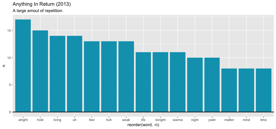
ggplot(TYM_Anything_In_Return_Lyrics_Count %>% head(15), aes(x=reorder(word, -n), y=n)) +
geom_bar(stat="identity", position="identity", fill ='#01A1BB') +
geom_hline(yintercept = 0, size = 1, colour="#333333") +
labs(title="Anything In Return (2013)",
subtitle = "A large amout of repetition.")
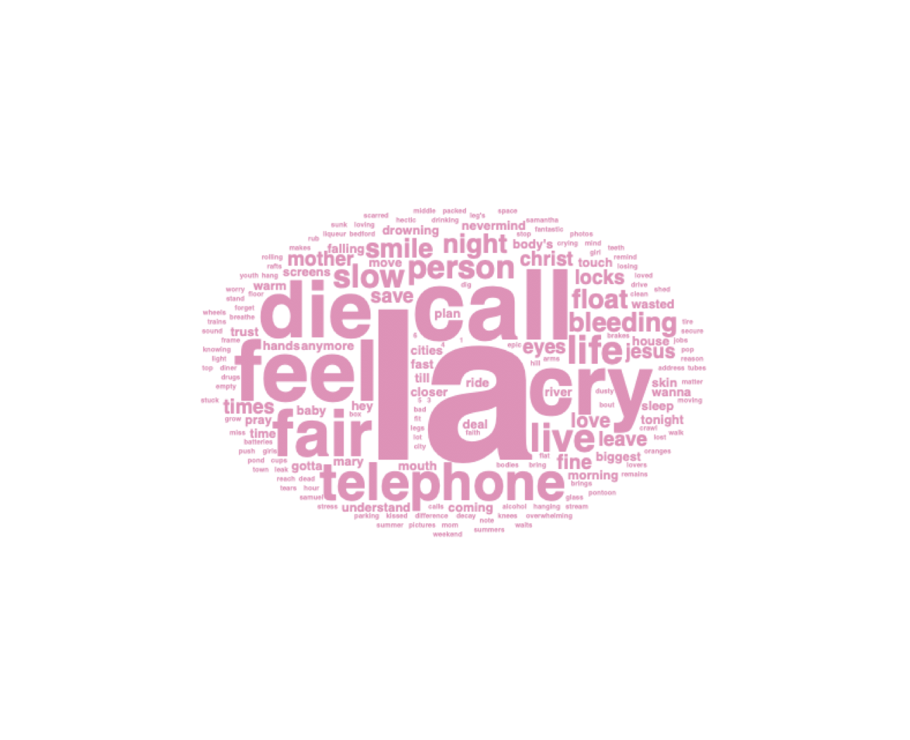
#June 2009
TYM_June_2009_Lyrics_Count <- TYM_June_2009 %>% unnest_tokens(word, lyric) %>%
anti_join(stop_words, by = 'word') %>%
count(word) %>%
arrange(-n) %>%
na.omit(TYM_June_2009_Lyrics_Count)
wordcloud2(TYM_June_2009_Lyrics_Count, fontFamily = 'Helvetica', color = '#EA8DB9', minRotation = 0, maxRotation = 0, shape = 'rectangle')
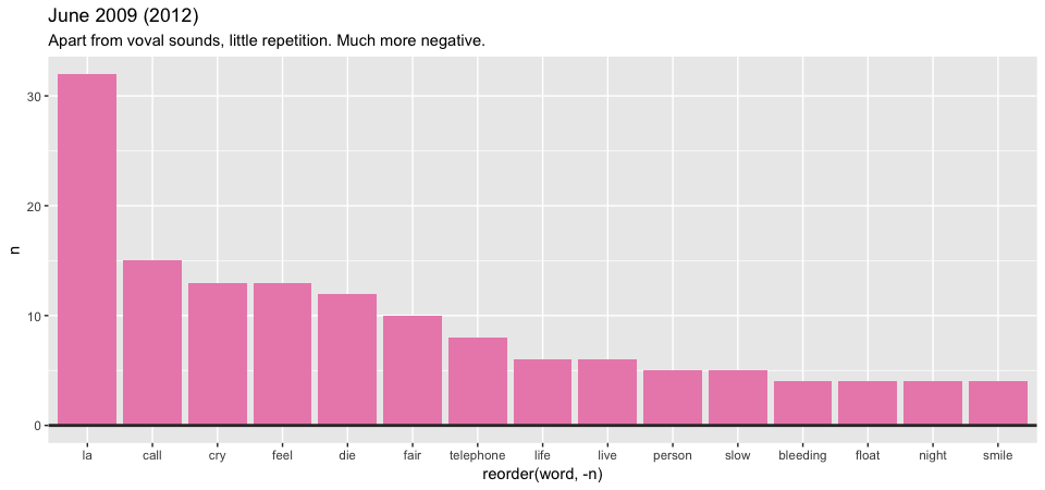
ggplot(TYM_June_2009_Lyrics_Count %>% head(15), aes(x=reorder(word, -n), y=n)) +
geom_bar(stat="identity", position="identity", fill ='#EA8DB9') +
geom_hline(yintercept = 0, size = 1, colour="#333333") +
labs(title="June 2009 (2012)",
subtitle = "Apart from voval sounds, little repetition. Much more negative.")
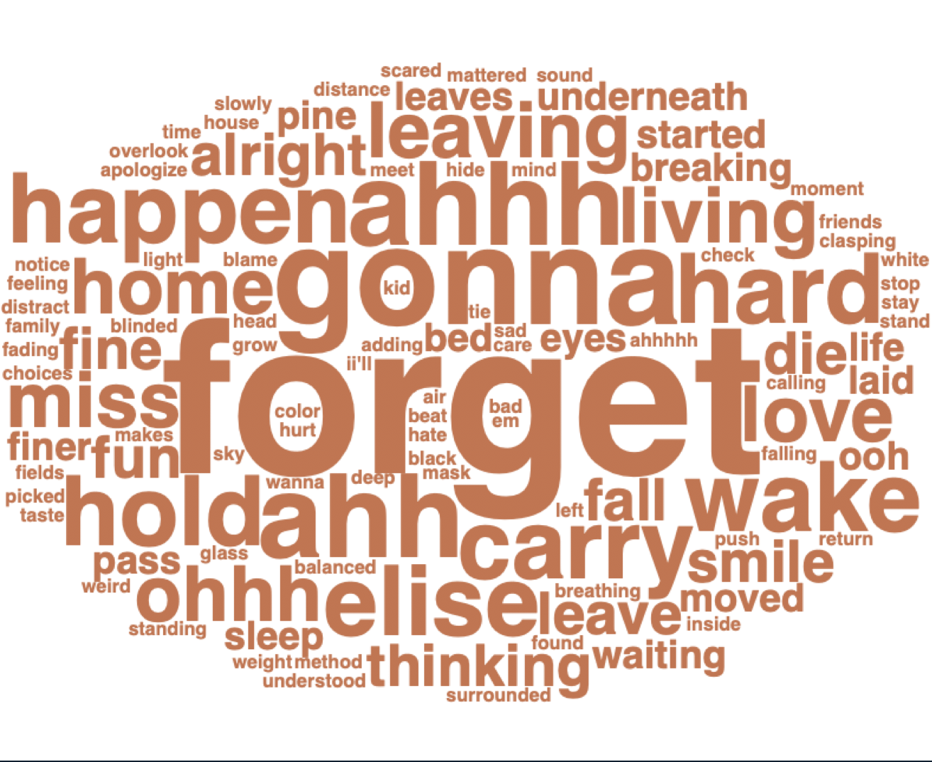
#Underneath The Pine
TYM_Underneath_The_Pine_Lyrics_Count <- TYM_Underneath_The_Pine %>% unnest_tokens(word, lyric) %>%
anti_join(stop_words, by = 'word') %>%
count(word) %>%
arrange(-n) %>%
na.omit(TYM_Underneath_The_Pine_Lyrics_Count)
wordcloud2(TYM_Underneath_The_Pine_Lyrics_Count, fontFamily = 'Helvetica', color = '#CB724A', minRotation = 0, maxRotation = 0, shape = 'rectangle')
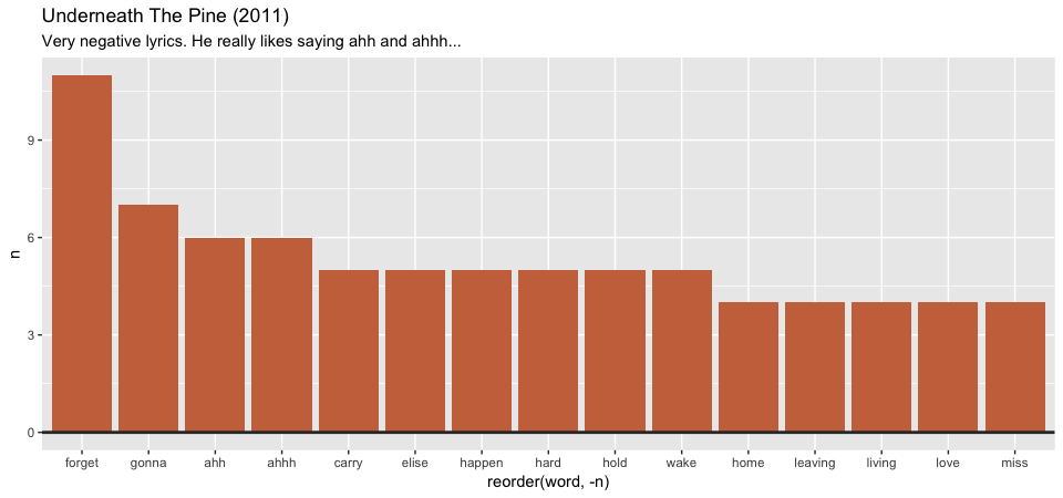
ggplot(TYM_Underneath_The_Pine_Lyrics_Count %>% head(15), aes(x=reorder(word, -n), y=n)) +
geom_bar(stat="identity", position="identity", fill ='#CB724A') +
geom_hline(yintercept = 0, size = 1, colour="#333333") +
labs(title="Underneath The Pine (2011)",
subtitle = "Very negative lyrics. He really likes saying ahh and ahhh...")
Chaz changes lyrical styles from album-to-album and we can see this reflected in the data. We can see that he's started to incorporate more vocal sounds and nonsense words, especially in Outer Peace. He's also incorporated more words relating to love (such as baby, love, and pleasure) in his later releases.
How do album sentiments change?
Now that we have seen the overall movements of joy in each album and the most popular words, we need to see how sentiment changes with each album as a whole. To do this, I used the NRC lexicon to find all words associated with sadness and found the percentage of lyrics that matched these words.
#List all sad words:
sad_words <- sentiments %>%
filter(lexicon == 'nrc', sentiment == 'sadness') %>%
select(word) %>%
mutate(sad = T)
sad_album <- TYM_All_Lyrics %>%
unnest_tokens(word, lyric) %>%
anti_join(stop_words, by = 'word') %>%
left_join(sad_words, by = 'word') %>%
group_by(Album_Name) %>%
summarise(pct_sad = round(sum(sad, na.rm = T) / n(), 4),
word_count = n()) %>%
ungroup
sad_album$pct_sad <- sad_album$pct_sad * 100
sad_album['year'] <- 1:6
sad_album$year[sad_album$Album_Name == "Outer Peace"] <- 2019
sad_album$year[sad_album$Album_Name == "Boo Boo"] <- 2017
sad_album$year[sad_album$Album_Name == "What For?"] <- 2015
sad_album$year[sad_album$Album_Name == "Anything In Return"] <- 2013
sad_album$year[sad_album$Album_Name == "June 2009"] <- 2012
sad_album$year[sad_album$Album_Name == "Underneath The Pine"] <- 2011
ggplot(sad_album, aes(x = reorder(Album_Name, year), y = pct_sad)) +
geom_bar(stat="identity", position="identity", fill ='#5C79BB') +
scale_y_continuous(labels = function(x) paste0(x, "%")) +
geom_hline(yintercept = 0, size = 1, colour="#333333") +
labs(title="Saddest Albums",
subtitle = "Overall, the albums become less sad.") +
xlab("Albums By Year") + ylab("% of Lyrics With Sad Sentiments")
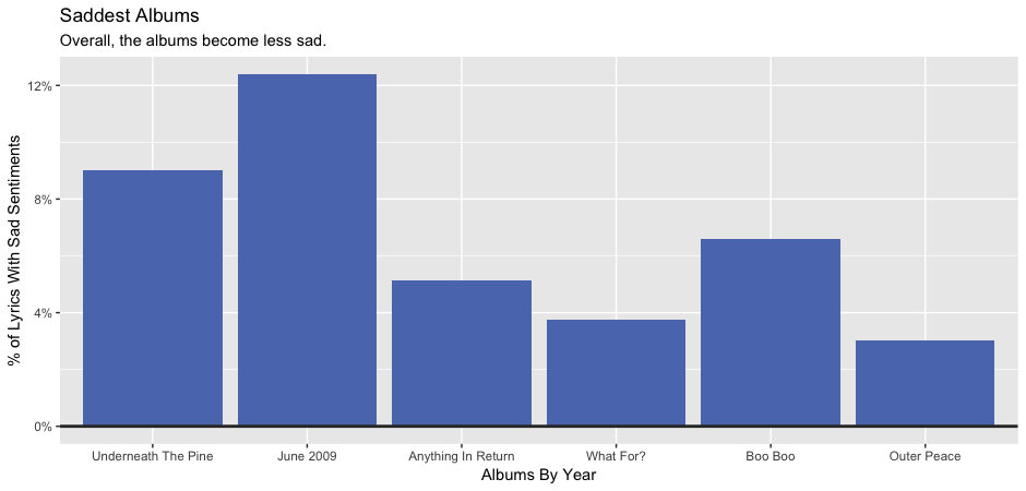
Apart from the two outliers, June 2009 and Boo Boo, the overall trend is that each new album contained fewer words associated with sadness than the previous release.
Conclusion:
Overall, we have found that Chaz's lyrics have become more joyful and that he has included more repetition in his more recent albums. Looking at Spotify data, this is backed up, showing a move to more joyful music. This supports my hypothesis.
Future Exploration:
Some future idea would be to look into different types of sentiment analysis and compare these with Spotify's findings. I'd also quite like to compare the popularity of the most danceable tracks from Spotify and LastFM to see what aspects of the song have the largest impact on popularity. How does the impact from the BPM, key, danceability, valence compare to the impact of the lyrical sentiment? This could be a good final project.