Chance the RappeR

A Musical and Lyrical Sentiment Analysis of Coloring Book Using R

By Blaine Williamson

Introduction + Hypothesis

As a music lover and avid Spotify user, I sought to analyze the musical and lyrical sentiment of an album using R packages that utilized Spotify's and Genius's APIs. Rolling Stones named Coloring Book by Chance the Rapper a top 50 album of 2016 stating, "The year's finest hip-hop album had a vision as radiant as its pink-sky cover art. Chance the Rapper's third mixtape combines radical politics and heavenly uplift to create life-affirming music that refuses to shy away from harsh realities. He uses the optimistic, joyful sounds of gospel choirs to soundtrack his hopes, fears and blessings, giving practically everything a spiritual hue. The album explodes with enthusiasm, as Chance embraces both the convoluted microphone mathematics of the old-school and the unpredictable melodic twists of the new. An electric dispatch from Chicago, Chance's infectious sing-song weaves together his faith, a city in crisis, his new daughter and the unique struggle of being the world's most famous unsigned musician." The wide array of lyrical content and musical beats made Coloring Book my go-to album for analysis.

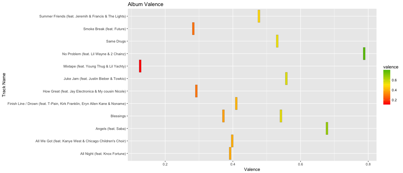
Spotify’s API provides a variable called “valence”, which is defined as "A measure from 0.0 to 1.0 describing the musical positiveness conveyed by a track. Tracks with high valence sound more positive (e.g. happy, cheerful, euphoric), while tracks with low valence sound more negative (e.g. sad, depressed, angry)." I wanted to compare the sentiment of both sound and word and how it correlated to popularity on the album. My hypothesis was that more popular tracks would have a higher valence (i.e. a more happy, cheerful sound) regardless of the sentiment of the lyrics. Even if the lyrical content was highly negative, I hypothesized that listeners would be drawn to musical positiveness over lyrical positiveness, and this would be evident in the tracks' popularity.

1. Spotify Data Frame

I first needed to make an app and get API credentials for Spotify. I loaded necessary packages, installed the "spotifyR" package from charlie86 on GitHub, and integrated my Spotify client ID and secret ID to access Spotify data. I then utilized the "get_artist_audio_features" function included in the spotifyr package to access data affiliated with Chance the Rapper as an artist on Spotify. I then removed row 4 of the data frame, the track "D.R.A.M. Sings Special," because it is a full feature song that does not include Chance the Rapper.

1. Genius Data Frame

I then needed to get API credentials for Genius. I loaded necessary packages and installed the "geniusR" package from josiahparry on GitHub. I then utilized the "genius_album" function for the Coloring Book album. I changed the name of the "track_title" to "track_names" in order to match the spotify data frame from above. I ensured the lyrics were characters within the data frame, and used the unnest_tokens function. I used stop_words to remove sentiment-free grammar, like "am," "we," "because," or "the," so as to get a more accurate lyrical sentiment later on. I merged my data frame with a sentiment data frame using the "bing" lexicon. I then merged the data frame to include track_name, track_n, line, word, and sentiment.

3. Visualizations

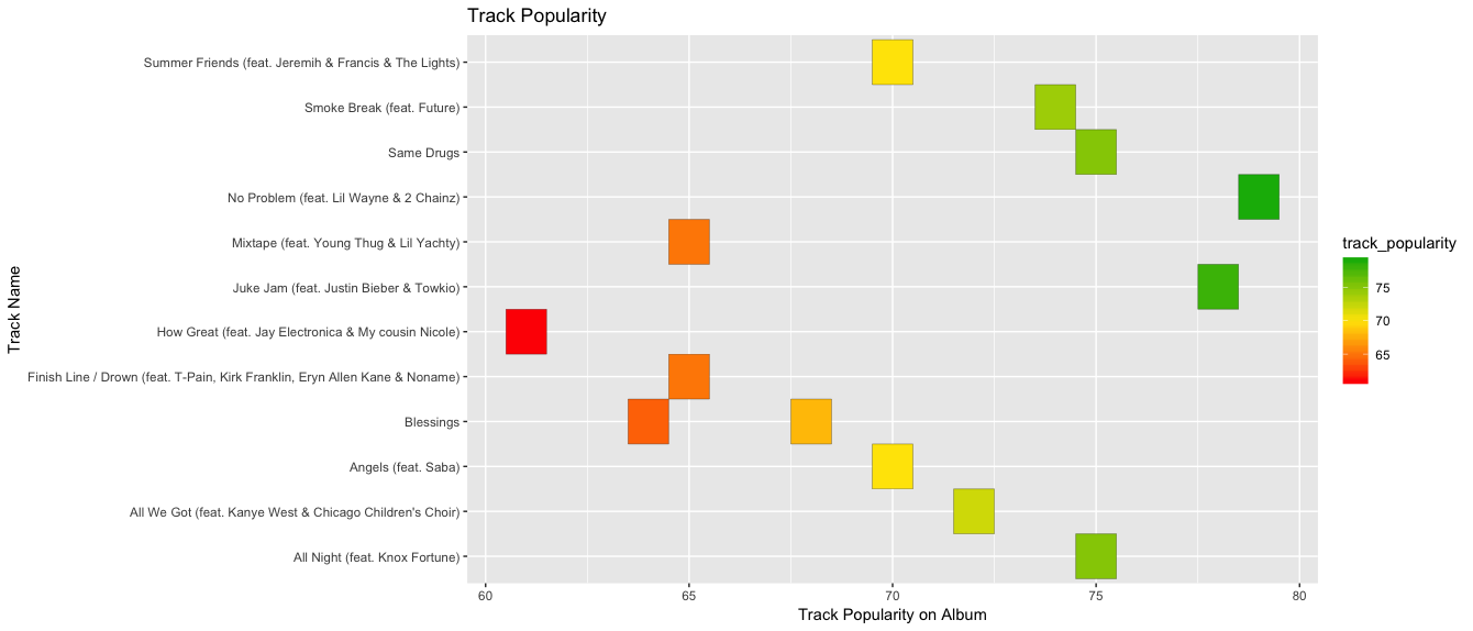
I then wanted to visualize the album's valence, lyrical sentiment, and track popularity to test my hypothesis. I chose a heatmap to compare the three. For the heatmap of the lyrics, I the midpoint is 0, representing a neutral lyrical sentiment. For the heatmap of valence, the midpoint is 0.5 because Spotify quantifies valence between 0.0 and 1.0. For the heatmap of popularity, the midpoint is 70 as a median of the lowest track popularity score (69, indicating the least popular song on the album) and the highest (81, indicating the most popular song on the album).

The Results:

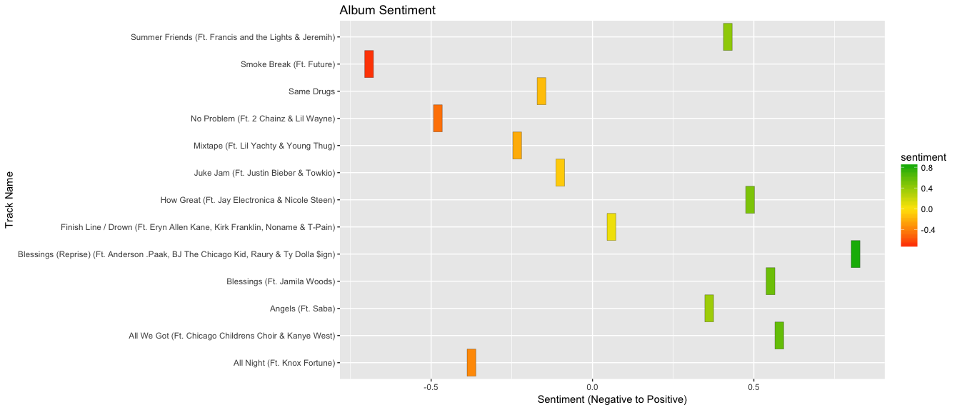
4. Conclusions

I hypothesized that more popular tracks would have a higher valence (i.e. a more happy, cheerful sound) regardless of the sentiment of the lyrics. Even if the lyrical content was highly negative, I anticipated that listeners would be drawn to musical positiveness over lyrical positiveness, and this would be evident in the tracks' popularity. My hypothesis is true, overall, made apparent by the above visualizations. The heatmap of track popularity looks much more similiar to the heatmap of valence, rather than the heatmap of lyrical sentiment at the top.

Most notably, "No Problem" is the second most negative song lyrically, but has the highest valence level. It is the most popular song on the album. Similarly, "How Great" is lyrically positive, but has the third lowest valence score on the album and is the least popular song overall on the album. On the contrary, "Smoke Break" is the most negative song lyrically on the album, has a lower valence score, and still remains relatively popular in relation to other songs on the album. Overall, music positiveness (high valence) matters to Chance the Rapper's listeners more than lyrical content. I also found it interesting how Chance the Rapper tends to be perceived as a very positive rapper, particularly because of his Gospel influences throughout his music. I found it interesting that Chance neared a 50/50 split on "happiness" both from a lyrical and musical standpoint.

5. Something extra...

After my analysis of sentiment and valence, I got to thinking how musicians, especially Chance the Rapper, communicate through more than just their music. I decided to run a sentiment analysis of Chance the Rapper's Twitter account to see if Chance's positivity translated from fans' earbuds to their newsfeeds. I installed the "rtweent" package from mkearney on GitHub and used the "get_timeline" function on @chancetherapper's timeline. I cleaned his tweets of retweets and links and merged the data frame with the sentiment data frame using the "bing" lexicon. I then visualized his 20 most used negative and positive words on Twitter.

The Results:

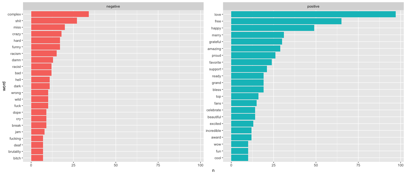
Chance the Rapper appears to be more positive than negative, at least when it comes to Twitter. Six of his top 20 negative words are swear words or varients of swear words, which could have previewed or followed something positive (i.e. cool shit, happy as hell).

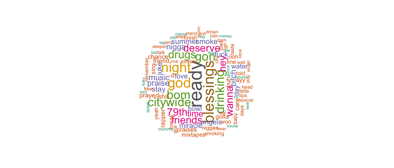
I then loaded the necessary packages for creating a wordcloud and compared the previous findings back to his lyrics on the Coloring Book album.

The Results:

I was surprised by the lack of overlap between the above visualizations, but it makes sense that the words he uses on Twitter would differ than the words he uses in his songs.